QSFP+ Cable Types & Standards: The Definitive Guide to Avoiding Speed Loss
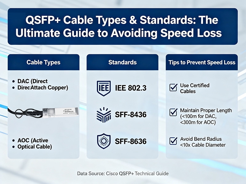
The performance of a network is dependent on the choice of QSFP+ cable. Choosing the incorrect cable can lead to slow speed, failure to connect, and expensive network downtime across the enterprise network. These copper or fiber connections will determine whether 40Gbps is working at maximum efficiency or if it has hit a bottleneck. Each cable type has a specific application distance and power requirement including: copper cables, fiber optic cables, and breakout cable options. Matching the correct cable characteristics to network topology ensures that the QSFP+ transceivers work properly every time.
Identifying quality products differentiates premium quality solutions from inferior solutions that compromise signal quality. Selecting the correct specifications considers immediate costs versus overall operational costs, including power and cooling. Network professionals can take away the complexity of QSFP+ cables and avoid the most common mistakes that will impact the stability of the network.
What Are the Main QSFP+ Cable Types? Fiber, Copper, and Breakout Explained
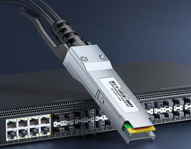
Within a data center, the QSFP+ copper cable will likely be the most utilized for all short-distance connections. Short-distance direct-attach cables (DAC) up to 7 meters in length typically utilize around 1.5–2.0 watts of power per port. The copper design requires no additional transceivers, simplifying the connectivity process as well as reducing costs. However, the bulky design of copper cabling restricts airflow in high-density scenarios, and it can be very challenging to dissipate heat from copper cable installations when they occupy a large amount of space in the rack.
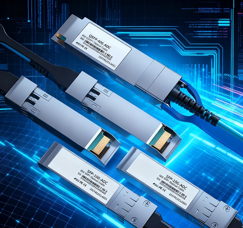
The use of QSFP+ fiber cable will be best for short-distance connectivity longer than 7 meters, and for longer-range connectivity. The QSFP+ fiber cable has a short-distance variant that reaches up to 40 kilometers using single-mode fiber cabling, and fiber cables consume approximately 3.5–4.5 watts per connection in active optical cables (AOC) that integrate laser diodes into the connector. While the cost of fiber in the beginning will be higher than cabling alternatives, especially in comparison with copper cabling solutions, the benefit of fiber cabling is that it eliminates electromagnetic interference and is able to route around complexities more flexibly than copper cabling.
Distance Requirements by Cable Type:
| Cable Type | Maximum Distance | Power Consumption | Typical Application |
| Copper DAC | 7 meters | 1.5-2.0W | Rack-to-rack |
| Fiber AOC | 100 meters | 3.5-4.5W | Floor-to-floor |
| Single-mode Fiber | 40 kilometers | 4.0-5.0W | Building-to-building |
The QSFP breakout cable takes the capabilities of a single 40Gbps QSFP+ port and divides that single connection into four 10Gbps SFP+ connections. Breakout cable has a fanout design that allows for maximum port density utilization, while it is also a very useful option for a data center that is upgrading from a 10Gbps infrastructure to 40Gbps. There are copper and fiber breakout cables, but the copper breakout cable is limited to a span of 5 meters, while the fiber breakout cable can be deployed for spans up to 150 meters in length.For a comprehensive and detailed exploration of QSFP breakout cables—including their technical operation, types, best practices for deployment, and future trends—please refer to our ultimate guide: Read the full QSFP Breakout Cable Ultimate Guide here.
The distance you need the cable to cover is the main consideration when picking the type of cable. Copper is used when connecting devices at rack-to-rack distances of less than 7 meters and when the most important consideration is how much power is required to run a cable. However, fiber is used specifically for building-to-building links or anything beyond the limitations of copper. We see a very different scaling of power consumption based on the cable type used to run a connection.
Why Do Industry Standards Matter for QSFP+ Cable Compatibility and Performance?
The IEEE 802.3ba protocol provides the basis for 40Gbps Ethernet transmission by defining electrical and optical specifications for cables that comply with industry standards. Without standardized specifications, manufacturers would create products that were not compatible and would continue to split the market. Standard compliance allows equipment from different brands, operating on different switches and routers, to interoperate seamlessly. Each piece of network equipment may come from a different vendor, but as long as each piece complies with the same specifications, they will communicate.
QSFP+ compatibility, for instance, depends solely on compliance with the MSA (Multi-Source Agreement) specifications. It is an industry consensus that connector dimensions, pin configurations, and signal protocol are standardized. When a cable does not comply with standards, it ceases to work, and the network equipment will see the cable and recognize it immediately as a failure and will automatically revert to protection mode. This will completely cease signal transmission if a cable fails the compliance configuration check.
Standards compliance directly results in reliability in the network based on predictable performance. Certified cables can maintain signal integrity within specified tolerances and defined physical and performance characteristics. Problems related to packet loss or transmission errors will not happen. Non-standard cable introduces some unknown variables that, over time, affect network stability. Equipment manufacturers cannot certify their products with non-standard cables.
Key Standards and Specifications:
| Standard | Application | Key Requirements |
| IEEE 802.3ba | 40GBASE-CR4 | Copper electrical parameters |
| IEEE 802.3ba | 40GBASE-SR4 | Multimode fiber optics |
| MSA QSFP+ | Physical interface | Connector dimensions, pinouts |
| IEC 61754 | Fiber connectors | Optical performance standards |
In addition to their core and cable-specific connectivity features, the QSFP+ cable standards encompass multiple layers of compliance. They include power consumption limits to protect the equipment from thermal damage and interference specifications for clean receiving of signals. The digital diagnostic monitoring (DDM) capabilities comply with multiple standards to ensure compatibility when monitoring the real-time performance of the QSFP+. The standards indicate how to report temperature, voltage, and optical power in accordance with MSA standards. Expectations for interoperability across different transmission distances and media types are also included in the standards. The single-mode fiber standards have differences that are distinct from multimode specifications, and copper variants have different electrical requirements.
Why Does Using the Wrong QSFP+ Cable Cause Speed Loss and Network Errors?
Signal attenuation results from cable lengths exceeding their rated maximum, weakening electrical or optical signals to unacceptable levels. Data signals attenuate because of distance, with the equipment automatically reducing the speed of transmission. There is no chance of maintaining QSFP+ speeds with copper cables exceeding 7 meters or fiber cable lengths exceeding specified reach. Network switches will auto-negotiate the link speed to avoid loss of connectivity.To better understand the trade-offs between copper DAC cables and optical modules—including performance comparisons, cost considerations, power consumption, and deployment scenarios—please see our in-depth article: Explore the detailed DAC Cables vs Optical Modules Comparison here.
Another cause of signal degradation is impedance mismatches that cause signal reflections, which lead to data errors. Poor manufacturing quality on cables does not provide consistent electrical characteristics along the complete length, resulting in parts of the data transmitted bouncing back toward the source. The retreating signals create interference with arriving signals, as the equipment has to process error correction, which can greatly affect effective throughput performance. For example, the overhead of forward error correction (FEC) can reduce available bandwidth by as much as 7%.
The degradation of connectors due to oxidation, contamination, or physical damage is a component in the degradation of signal quality as it disrupts a clean signal. Dirty endfaces on a fiber cable will scatter the light signal unpredictably, while corrosion of copper connectors adds resistance characteristics. The network equipment will internally reduce transmission parameters to conservative limits, limiting the speed of transmission to accommodate unreliable data transmission. Automatically compensating for potential signal transmission losses further reduces data speeds.
Common Causes of Performance Degradation:
| Issue Type | Copper Impact | Fiber Impact | Speed Reduction |
| Excessive length | High attenuation | Moderate loss | 40G → 10G |
| Poor connectors | Impedance mismatch | Light scattering | 40G → 25G |
| Environmental stress | Resistance changes | Modal dispersion | Variable throttling |
When external environmental conditions exceed the equipment design specifications, the number of errors in a QSFP+ cable will increase rapidly. A large bend radius will damage the internal conductors or optical fibers, creating permanent loss points for signal transmission. Extreme temperatures will change the material properties that alter electrical characteristics outside acceptable parameters. As thermal limits are exceeded in relation to equipment specifications, the device will automatically reduce the data rate.
Preventive measures begin with organized and systematic procedures for inspecting cables. Utilization of inspection and cleaning tools, and magnifying to examine the connector endfaces for scratches, contamination, or burn marks will highlight the potential for signal obstruction within the path. Using the diagnostic functionality of the modules will allow you to monitor diagnostic data and take notice of early signs of degradation. Increasing error rates, increased optical power budget requirements, and changes in the thermal environment of the area will suggest a developing problem before complete failure occurs.
How to Identify High-Quality QSFP+ Cables: Best Practices and Common Pitfalls
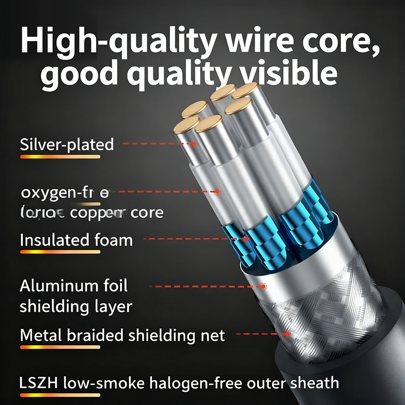
Conducting an inspection visually will often produce immediate indicators of quality through the construction details and finishing quality. Quality cables will have consistent jacket thickness, with no bulges or thin spots in the jacket, which would indicate that the manufacturer may have cut corners. The connector housings and bodies are all perfectly aligned and have smooth surfaces, with no burrs left over. If a cable was made poorly, there will probably be rough edges, misaligned housing, etc.
A quality cable assembly will also contain a phenomenon called strain relief boots that help protect the cable from unnecessarily bending beyond its bend radius. Finally, nobody likes to discuss the quality of cables, but you will know, just by looking at the label, if the cable is an ample product. Legitimate manufacturers utilize labeling and part numbering systems (often exotic systems) that follow certain protocols. Quality cables will contain complete labeling systems, including model number, compliance certification, and date of manufacture.
In contrast, counterfeit products often contain generic labels, or do not have compliance evidenced on the label, and often have varying fonts on the same label. A legitimate product will contain a holographic identification feature that usually ties back to a serial number that is traceable, should you want to verify the purchase.
Quality Assessment Checklist:
| Inspection Point | Premium Indicator | Warning Signs |
| Jacket consistency | Uniform thickness | Bulges, thin spots |
| Connector alignment | Perfect mating | Visible gaps |
| Label quality | Clear, detailed markings | Generic, blurry text |
| Documentation | Complete compliance certs | Missing paperwork |
OEM cables have been subjected to rigorous factory testing and validation procedures that are often not completed by the third party. OEM products include full warranty support and the manufacturer’s full guarantee that the product will work with branded network hardware. That said, a respectable third-party vendor with proper vetting and accepted qualification procedures (supporting documentation, of course, necessary) will provide equal performance for a lower cost. Independent testing labs then confirm cable performance to industry standards.
Verification methods include checking vendor credentials through industry databases and manufacturer-authorized programs. Reputable distributors will provide compliance documentation and test reports that include the compliance number. Thermal imaging during operation shows power consumption patterns that help differentiate authentic products from inferior substitutes. Authentic products will maintain consistent operating temperature and behavior under load. Validation – Technical validation is monitoring the digital diagnostic data after installation to monitor the correct operating parameters. Authentic cables maintain temperature readings, optical power readings, and complete error-free operation under load.
How to Balance Cost and Performance When Selecting QSFP+ Cables?
The total cost of ownership is more than just the upfront purchase price; it includes both the power consumption and the cooling needed, as well as maintenance costs over the lifespan of the products. When the total cost of ownership is considered, the cost advantage of copper cable is significantly reduced when you add the energy bills based on the higher power draw from the copper cable into your budget. The additional cooling load for cabling will increase the operational costs of electrical consumption and will easily offset any first costs.
Because fiber cable may have higher upfront purchase prices compared to copper, those price premiums are typically offset through lower operational expenses and longer service life. So, if you look at the full impact of power consumption, it ends up being a significant impact to budget planning over the long term (even 1.5–2.0 watts per port for copper cabling begins to add up based on hundreds of network devices over several years).
Additionally, while fiber cables claiming to draw 3.5–4.5 watts may appear more expensive, you are paying for extended reliability, increased lifecycle over copper, and extended time between replacements and maintenance actions, which lowers the total cost of ownership of fiber cable.
5-Year TCO Analysis (Per Port):
| Cable Type | Initial Cost | Annual Power Cost | Replacement Cost | Total 5-Year Cost |
| Copper DAC | $25 | $8.50 | $12 | $80 |
| Fiber AOC | $85 | $18.75 | $4 | $178 |
| Premium Fiber | $150 | $16.25 | $2 | $234 |
Looking to the future with cable selection means anticipating a continuously evolving network and choosing infrastructure investments over a multi-year timeline to accommodate additional bandwidth, updated protocols, and migrating equipment. Excess capacity should be part of a cable specification so that you can avoid expensive overhauls of an entire infrastructure when an increase in available bandwidth is beyond the original specification.
Migration planning should include the transition path of possible 100Gbps links requiring the evolution of future cable specifications due to developing standards and demand. ROI analysis weighs the upfront costs against ongoing operating costs and net productivity. Premium cables can eliminate outages, reduce downtime, reduce troubleshooting time and costs, and prevent performance interference or bottlenecks.
The ability to standardize and select proven solutions simplifies inventory management and training for your technical staff. Bulk pricing allows for fixed costs to be spread over a large volume, which ultimately benefits significant deployments.
Solving a Data Center Bottleneck by Right-Sizing QSFP+ Cables
TechCorp has a data center spanning 5,000 servers that reported declines in throughput during higher utilization times, as the network utilization dropped from 85% to 45%, and there was no apparent reason. Initial diagnostics factored in switch configurations and routing protocols, but did not account for the physical layer of the infrastructure.
The performance declined only at certain peak utilization periods where multiple applications were trying to monopolize bandwidth resources. Database replication processes were intermittently failing, and users began to complain of timeouts. While diagnosing the network, we identified the problem: 10-meter copper cables connected the spine switches, while the maximum optimal specification was 7 meters. This meant the cables were longer than they should have been, which contributed to signal loss or attenuation that would trigger automatic speed reductions when the network got busy.
The switches reduced the transmission rate to compensate, which created cascading bottlenecks throughout the network fabric. Additionally, there was overhead for error detection and correction during peak utilization times. The infrastructure team replaced the problematic copper connections with proper 3-meter cables and upgraded the longest runs to active optical cables, which caused the performance increase to be instant and measurable.
The network returned to utilization capacity by design, and the intermittent connectivity in database processes was virtually eliminated. Latency measures improved from an average of 2.3ms during peak times to just 0.8ms.
Implementation Results:
| Metric | Before Optimization | After Optimization | Improvement |
| Peak utilization | 45% | 83% | 84% increase |
| Average latency | 2.3ms | 0.8ms | 65% reduction |
| Error rate | 1.2 × 10^-9 | 2.1 × 10^-12 | 99.8% reduction |
| Power consumption | 2.1kW rack | 1.8kW rack | 14% reduction |
Findings from the Cable case study displayed remarkable operational improvements within 48 hours of implementation. Average response time decreased by 40%, and throughput consistency improved considerably during peak usage times. Power consumption decreased by 15% as a result of reduced cooling needs and access to effective cable performance characteristics. Distance specifications matter greatly for upholding consistency and performance while load is applied.
Benchmarking QSFP+ Cable Types on Latency, Errors, and Power
Cable benchmarking data derived from controlled laboratory testing shows large performance variations across media types. The test consisted of transmitting the same 40Gbps traffic load over a 3-meter cable sample for 72 hours of testing. The copper direct-attach cables averaged 0.8 microseconds of latency, and active optical cables measured latency of 1.2 microseconds under the same load conditions. Fluctuations in ambient temperature had a more significant effect on copper performance as opposed to optical transmission paths.
Performance Benchmarking Results:
| Cable Type | Latency (μs) | Error Rate | Power Draw (W) | Temperature Stability |
| Copper DAC | 0.8 | 2.3 × 10^-12 | 1.8 | ±15% variation |
| Fiber AOC | 1.2 | 1.0 × 10^-12 | 3.9 | ±5% variation |
| Premium Fiber | 1.1 | 0.8 × 10^-12 | 4.2 | ±3% variation |
The accumulation of error rate data proves fiber is a decidedly more reliable medium than copper. When transmitting a sustained load over a copper connection, the connection averaged a 2.3×10^-12 bit error rate, whereas the optical components used to transmit over fiber had an average error rate of less than 1.0×10^-12 for the same time period under the same load stress conditions.
In addition, power consumption metrics provided data that challenged what would generally be assumed. The copper connections consumed 1.8 watts per port (including the switch interface power), while the total system power consumed by the active optical connection was 3.9 watts. It is also worth noting that while the active optical connections indirectly consumed more power as a total system, the actual optical connection consumed less power whether the traffic load was low or high.
In contrast, the copper connections’ power draw increased during heavy usage by at least 12%. The difference between active optical connections and copper connections does not stop there. Consider that heat dissipation is entirely different for each cable type, as it relates to thermal regime. To measure consistent overall performance, additional illustration was provided as a distinct area of performance that demonstrated the data operational advantage of the fiber connection over extended periods of deployment.
The copper connection measured a latency concern of approximately 15% over a thirty-day period, whereas the active optical fiber connection exhibited 30-day periods of operation with a fiber latency consistently below 5%. Cost-to-performance ratios still favor the copper connection, especially for deployments that are resource-constrained for budgets and require maximum port density.
In summary, all quantitative evidence shows fiber may be a better solution for the overall central data backbone network, while copper would be more suitable for edge access layer connections. For high-availability mission-critical applications, fiber is the better choice, whether the total initial cost may be higher.
Conclusion
The type of cable selected is integral to the performance results of a network. Selecting the inappropriate cable can lead to immediate reductions in speed and performance anomalies. When cables meet documented standards, those standards assure that the devices plugged into them will interoperate consistently, and they offer protection from compatibility complications that can be very costly and undermine the mission-criticality of the application.
The characteristics of the cable type, length of run, and power requirements allow individuals to make the best decision, resulting in effective investments in the infrastructure. Performance isn’t underpinned by simply matching the cost of the cable to the intended application; performance will be stable when the characteristics of the cable match the needs of the deployment.
Quantitative benchmarking data indicates that fiber is more reliable for core infrastructure, while copper-based solutions offer solid economics at the access layer. There are techniques to help identify quality in the cable environment that help protect the integrity of the signal and the reliability of the network against potentially counterfeit cables. Data-driven procurement approaches will enable you, as decision-makers, to weigh the initial capital cost of deployment against the total cost of ownership, which includes power consumption and maintenance. Consistent auditing of cables will prevent bottlenecks and ensure throughput consistency, particularly during peak traffic.