How to Calculate Fiber Optic Cable Attenuation: Stop Overpaying for Wrong Distances
Have you ever ordered a large quantity of fiber optic cable for a major project only to have all work stop because the signal wouldn’t maintain integrity? Too often, buyers do not perform basic attenuation tests before they begin installing fiber optic cabling, which causes them to add costly splices or purchase premium-grade fiber optic cables that are overkill for the distance they need. Using this simple mathematical formula allows you to determine your link budget early in the project so you can determine the appropriate safe operating range and save yourself from unnecessary expenditures on rewiring, splices, or excess reels of fiber optic cable.
Why Does Wrong Attenuation Ruin Your Fiber Optic Cable Budget?
Buyers tend to buy the most economical fiber optic cable with the expectation of data transmission being both fast and reliable; however, the many points of signal loss on the cable cause the signal to deteriorate. This is primarily due to insufficient attenuation calculations when installing the cable. In addition, it also creates considerable rewiring costs, often in excess of $5000 in one instance. Manufacturers who use short runs in their factory operations often fail to perform these calculations.
As a result, they typically have multiple splices in the same run, leading to as much as 300% in added costs in a single day. This results in managers buying low-loss fiber optic cable that is far too expensive to use on short runs. Similarly, there is a tendency to buy high-quality reels of fiber optic cable for long runs, only to have them sitting idle on a simple run, wasting cash and delaying projects while waiting for the corrections to be made.
Similarly, in a larger warehouse with 400 meters of bridge rack, it is likely that no one will check when bends are made, which can lead to 10G network issues. Therefore, there could potentially be weeks of delays due to complete reworking of that transmission chain. These instances occur frequently in office-based construction projects as well as with factory connections. However, there is a method to determine the best fiber optic cables for your installation by performing the initial calculations—minimum distances are best suited for cost-effective multimode, and maximum distances are best suited for single-mode fiber optic cable without excess.
By following the above guidelines, you should save a considerable amount of money on your fiber optic installations.
 How Can You Add Up Fiber Optic Cable Loss in 1 Minute?
 How Can You Add Up Fiber Optic Cable Loss in 1 Minute?
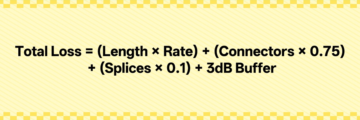
To quickly calculate the total loss of fiber optic cable within a minute’s time, simply multiply the distance of the fiber by the cable’s loss per kilometer, then add the amount lost due to various connector and splicing connections, and also include the overall safety buffer (3 dB). Because of the many external factors present, including accidental bumping, dust accumulation, and signal degradation over time, the 3-dB buffer provides a safety net against the unexpected, including problems related to cable breakage or splicing, connector ingress, or slow degradation of lasers being used in equipment. Thus, there is sufficient margin to keep the fiber link from failing without requiring the use of fixed repair figures.
At 1550 nm, single-mode fiber cables typically suffer approximately 0.2 dB of loss for every kilometer, while multimode OM3 and OM4 cables suffer approximately 3.0 dB/km (TIA standard maximum of 3.5 dB/km conservative calculation value) when connected at 850 nm. Each connector incurs a maximum of 0.75 dB of loss according to the Telecommunications Industry Association (TIA); however, when working with high-quality data centers, the loss per connector should remain below 0.3 dB to provide additional margin, and the loss per splice will vary from approximately 0.10 dB to as little as 0.02–0.05 dB depending upon the quality of equipment used to perform the splicing process. Therefore, the losses associated with installing these connectors will become greater as the total distance of the cable run increases.
Using traditional methods, if the distance is more than 40 km for single-mode or more than 500 m for multimode fiber, then dispersion will begin to adversely affect the signaling capacity of fiber optic cables because dispersion will smear the shape of the signal. Thus, contact one of the manufacturers of fiber cable for specific information to check to ensure you are operating within their specifications. If you are using long-range modules over short-distance fiber cable (less than one km), it is essential to utilize attenuators to prevent damage to the receiving devices.
For example, the use of a 5-km single-mode fiber cable at 1550 nm will only create a loss of 1 dB due to the length of the cable, therefore indicating that the low loss provided by low-loss standards is beneficial for extended distances. However, 1550 nm acts as a magnifying glass for bend defects. As an example, if you are inspecting the acceptance of a 1550 nm fiber optic cable and find that the loss is 0.5 dB greater than the loss associated with the same length cables operating at 1310 nm, this indicates that the fiber is in too tight a radius, which can be identified quickly by conducting a dual wavelength comparison to quickly locate defects associated with the bending conditions.
Walk Through a Real Example
 Walk Through a Real Example
The total cable loss for the distance of 3 km between the two connector points and the single splice will be: 0.2 dB/km (cable loss) x 3 km = 0.6 dB total loss + 1.5 dB from the two connectors + 0.1 dB due to the splice = a total of 2.2 dB in loss (based on cable loss) + 3 dB for the buffer (to remove the excess loss) = 5.2 dB total loss.
We tested a large data center installation based on the TIA/EIA 568 standards, which exhibited a total loss of 8.5 dB initially (through testing methods similar to these). After doing some extensive cleaning of the fiber end faces and replacing a bad splice, the installation achieved a total loss of 4.9 dB, and production was able to proceed without having to pull any new cables. Many of the 2-3 dB of recovery were due to cleaning the fibers that had been contaminated by dirt.
Therefore, always perform testing with an optical power meter before considering a job complete (to ensure compliance with the ITU-T G.652 guidelines, which specify that the maximum allowable loss for a 1550 nm system is 0.21 dB/km). Projects like this tend to perform well due to the low inherent losses of the 1550 nm wavelength, but it is important to remain vigilant to potential loss due to macro-bending sensitivity and to mitigate this issue by observing maximum turn radii when handling installations. 1550 nm acts as a magnifying glass for bend defects.
Please compute these calculations in your mind (early) and verify the determinations before they become an issue. In addition, avoid falling into the trap of assuming that the specifications for a given cable alone determine its performance.
Color Zones for Quick Decisions
 Color Zones for Quick Decisions
Use the calculated loss numbers as a basis for your decisions regarding the light module’s power budget, which can typically be found on the module manufacturer’s datasheet. For example, a 10G LR Module may have a Tx Min Power of -8dBm and an Rx Sensitivity of -14dBm (this provides a 6dB power budget), so it is important to consider the 3dB buffer.
To determine the proper module to use, first, find the budget from the module manual. Second, total your entire cable and connector losses to see if your total loss falls below the 3dB threshold for the 10G LR Module. If there is less than a 3dB difference (9dB loss vs. 11dB budget), you should upgrade to long-distance 10G modules or cut splices in order to create more room between your total loss and the power budget.
In this way, you can greatly increase reliability. For instance, if you calculated a 9dB loss and an 11dB budget, you have a 2dB spare margin, so instead of purchasing a $1,800 repeater, you would simply replace the module for approximately $250 and maintain your data throughput. If you see total losses of less than 7dB in comparison to the power budget, you are in the green zone and can expect many years of reliable service from that combination.
All losses from 7 to 11dB compared to the power budget would have signs of potential issues and would require careful attention to assure that you have pristine ends or to upgrade the module to one that would yield quick payback on elimination of repeaters. Should you have losses of greater than 11dB compared to the power budget, a complete redesign should be undertaken based on power budget decision zones, not Fluke Network’s testing standards.
What’s Your 2km Rule for Fiber Optic Cable Wavelengths?
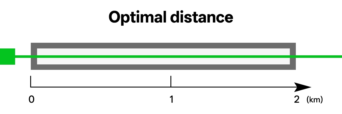 What’s Your 2km Rule for Fiber Optic Cable Wavelengths?
Choose connection types based on distance or speeds rather than strict 2 km connections. For connection types of 10 Gbps to 300 m, use multimode cables, e.g., OM3 and OM4, because the transceivers for these types cost between 1.5 and 5 times less than traditional devices; e.g., $16 for a 10G SFP module, versus above $34 in true market quotes for a 10G LR module. This makes them ideal for projects with limited budgets.
When running connections from 300 m to 2 km, switch to single-mode OS2; while prices may initially seem attractive for multimode, per IEEE standards, multimode cables will not support 10G from over 300 m. When using single-mode OS2 connections, although you pay a little more for the modules, they can provide substantial savings overall, due to their longer usable length compared to multimode.
For instance, on a 1.5 km 10G floor in a data center, OM4 only supports 400 m utilization of the cable per IEEE; going beyond that distance was maximizing the potential for degraded transmission quality. At this time, some teams that were in close proximity to the limits of their system capabilities were simply ignoring the expense associated with using single-mode OS2 connections; instead, they focused on utilizing fewer and less expensive multimode connections, thereby reducing the total costs of their systems by 25% by eliminating unnecessary excess purchases.
For all connections that exceed 2 km, primarily between buildings, OS2 single-mode connections should be utilized. There are multiple reasons for this: the average material costs for OS2 single-mode connections are lower than for multimode connections, the average number of transceivers or devices per kilometer of each type are higher for OS2 connections than for multimode connections, and the lower attenuation rates at 1550 nm wavelengths compared to 1300 nm provide additional cost-effectiveness overall.
In addition, hospitals typically use multimode cables for short but highly accurate signals at manageable costs, while oil companies have a tendency to run multimode cables up to verified cable maximum lengths before converting all future lengths into single-mode; this creates another opportunity for the creation of savings associated with the high installation costs of a single-mode cable system installed in extremely harsh conditions. When planning your installation projects, match your speed requirements to the distance your cable will span, and you will avoid pitfalls and overspending caused by defective optical fiber ends or poor optical fiber bends.
What Hidden Killers Wreck Fiber Optic Cable Links?
 What Hidden Killers Wreck Fiber Optic Cable Links?
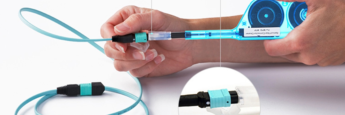
Keep one-click cleaning pens available before every connection to ensure that the ferrules of your connectors do not have smudges or dirt on them. You will see a 2 dB increase in loss from just having a smudge on the ferrule connector, which will cause your data transmission to go from 10G to 1G. Inspecting every end with bright light before connecting it to the other end will save you, on average, $5,000 each time you have to send a technician to troubleshoot a drop in signal levels due to smudges.
Cleaning the ends of the connectors nightly in a logistics hub that adheres to TIA/EIA guidelines creates reliable connectors with insertion losses in the range of 0.2 dB to 0.5 dB per connector and virtually eliminates potential downtime. Bends that are tighter than what the cable was designed for can create macro-bend damage with insertion losses of 2 dB due to excessive strain on the cable, which results in signal attenuation at unexpected times.
Installers should always adhere to the specifications outlined by IEC 60794, which state that static bends must be a minimum of 10 times the cable’s outer diameter and that bending is allowed during pulls to 20 times. Marking the minimum bending radius of the cable on the reels allows the installer to avoid having to worry about excessive strain on the cable and causing problems with your installation.
When installing connectors, always use like colors for all connectors (for instance, use blue UPC with blue UPC connectors). When installing the blue UPC connector into the green APC connector, you will create 8-degree angle ferrules and lose your connection because of misalignment. Standardizing your colors from end to end will help eliminate night failures like what happened in the example mentioned in the previous paragraph.
Taping color codes to your toolboxes and using them to install your connectors will help protect the connectors against the weather and make fragile installations less likely to occur.
How Do RFQ Requirements Protect Fiber Optic Cable in Tough Spots?
 How Do RFQ Requirements Protect Fiber Optic Cable in Tough Spots?
| Parameter | Indoor Spec | Outdoor Spec |
| Sheath | LSZH (low-smoke zero-halogen) | PE with stainless steel armor (rodent-proof) |
| Tensile Strength | Long-term <5% strain; short-term up to rated ultimate | Same, with 500N long/800N short per Kaiflex standards |
| Temp Range | -20°C to +60°C | -40°C to +70°C operation |
| Other | Water-blocking gel fill | Anti-UV, gel-locked seals, G.652.D fiber to eliminate 1383nm water peak for stable low loss in humidity |
High humidity in cable joint boxes and that amount of dust will lead to cable joints degrading faster than regular cables. When purchased with specifications mentioned, vendors must ship equipment ready for deployment, as with other network providers who were still working to get replacements with a basic jacket.
The high humidity will also allow for moisture to enter into the critical joint boxes. The factory runs produced consistently for the last year due to the existence of this 0.2 dB/km margin in addition to using gel fill when producing the cables.
Tropical storms are a serious threat to the integrity of cable poles, and cables produced with gel joints proved to be much more durable in storms than the poorly constructed bare cables on poles during the typhoons that hit Taipei during late 2021. Utility crews working to maintain their cable connections in storms were able to keep them operational.
When manufacturing using a factory floor temperature of 50°C, the outer sheath of the cables will crack without the existence of an anti-UV jacket, and therefore, when you have properly manufactured cables with a set standard, the vendor will be willing to provide you with the highest level of quality and product life in the industry.
How Do OTDR Steps Trap Fiber Optic Cable Buyers?
 How Do OTDR Steps Trap Fiber Optic Cable Buyers?
Don’t just ask for PDF images of your OTDR to place an order. Require suppliers to provide .sor-format OTDR output files, not photoshopped PDF images with hidden event spikes or smoothed traces. Weak suppliers will sell defective spools and bury defects in the fibers, whereas an analysis of the raw .sor output files allows you to confirm splice losses of less than 0.1 dB per direction (based on bi-directional analysis) regardless of any inconsistencies in how defects showed up as “pseudo-gain” in one direction when analyzing both directions.
Not just average dB/km, because if micro-cracks are present, they would also appear as a series of spikes along the length of the fiber optic cable. When reviewing raw .sor OTDR data, any non-connector event with a splice loss greater than 0.2 dB should be flagged as a potential fiber failure.
Comparing our efficiency on the fiber optic spools removed will allow you to quantify your freight savings. More than 15% of “bad lots” are known as “back-out lots”, due to how poorly they were manufactured by telecom companies, and not due to the way they were tested.
These clauses can save thousands of dollars on fiber returns, as many shippers have been able to return hundreds, if not thousands, of defective spool lots. Use the bi-directional averaging method to spot and manage directional losses.
Reference Sources
- Optical fiber – Wikipedia – Explains 1550nm macro-bend sensitivity as “magnifying glass for defects” vs 1310nm, matching article’s dual-wavelength bend testing method.
- Fiber-optic cable – Wikipedia – ITU-T G.652 specs (0.21 dB/km @1550nm SMF, 3.5 dB/km max OM3/OM4 @850nm), directly supporting article’s conservative 3.0 dB/km calculation.
- Calculating Fiber Optic Loss Budgets – FOA – Standard 3dB safety buffer, connector loss 0.3-0.75dB, splice loss 0.02-0.1dB, identical to article formula.
- Bi-Direction Testing with an OTDR – Fluke Networks – OTDR .sor files, bi-directional splice averaging <0.1dB, pseudo-gain detection, matching article’s supplier verification steps.
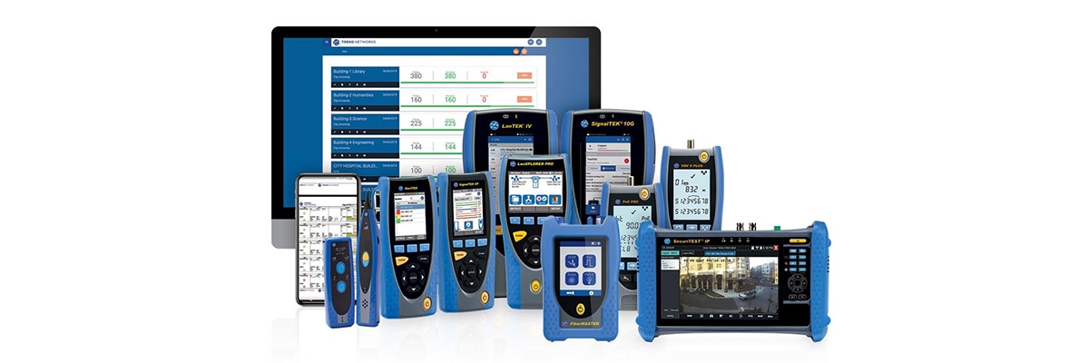
- Fibre Optic Cabling Loss Limits – TREND Networks – TIA-568 power budget zones (green <7dB margin, caution 7-11dB, redesign >11dB), confirming article’s color zones as industry practice.
- IEC Standards List – Optical Fibers – IEC 60794 bend radius (10x OD static/20x dynamic), IEC 60793-1-40 attenuation measurement, supporting RFQ specs and macro-bend warnings.